
Mantispy in ten minutes#
This page runs an image-based profiling screen from the raw object to a mechanism call, on one dataset, in one narrative. Every analytical step names a biological question, runs a few lines, draws a figure, and reads it back off. The other tutorials each take one of these steps in depth; here the point is the whole shape of the workflow.
Everything is a scverse object. adata.obs records where each profile came from, adata.var records what each
feature measures, and adata.uns["mantispy"] holds every result table. scanpy’s PCA, neighbours and embeddings
work on it unchanged, so no result exists only in a notebook variable.
import matplotlib.pyplot as plt
import numpy as np
import scanpy as sc

import mantispy as mt
import plotly.io as pio

pio.renderers.default = "notebook_connected"
A screen in one object#
BBBC021 is the field’s reference compound screen: MCF-7 cells, 38 compounds at one to seven concentrations, with
published mechanism-of-action labels. mt.ds.bbbc021() downloads and caches it, and hands back an ordinary
AnnData.
adata = mt.ds.bbbc021()
adata
AnnData object with n_obs × n_vars = 632 × 467
    obs: 'Metadata_Plate', 'Metadata_Well', 'Metadata_Compound', 'Metadata_Concentration', 'Metadata_MOA', 'Metadata_CellCount', 'Metadata_SiteCount', 'Metadata_Control', 'Metadata_Perturbation'
    var: 'object', 'feature_group', 'feature', 'channel', 'scale', 'angle', 'gray_levels', 'radial_bin', 'params', 'is_feature'
    uns: 'mantispy'
    layers: None (.X)
Rows are wells, columns are CellProfiler features, and every Metadata_ column in obs says what a well is: its
plate, its compound and concentration, its mechanism label, its cell count. Nothing here is mantispy-specific yet.
A scanpy user already knows this object.
Is the data worth analyzing?#
Before any modelling, two questions decide whether the screen is usable: do treated wells look different from the negative controls at all, and how much of what we see is the plate rather than the biology? We put every plate on the scale of its own DMSO wells, keep the informative features, and look at a PCA.
mt.pp.normalize(adata, method="mad_robustize", by="Metadata_Plate", reference="negcon", keep_raw=True)
mt.pp.feature_select(adata, na_cutoff=0.0)
adata = mt.pp.subset_features(adata)

sc.pp.pca(adata, n_comps=30)
adata.obs["Well type"] = np.where(adata.obs["Metadata_Control"].to_numpy(), "control", "treated")
sc.pl.pca(adata, color=["Well type", "Metadata_CellCount"], ncols=2, show=False)
plt.show()
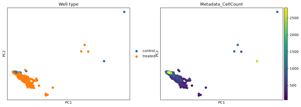
The controls sit together and the treated wells fan out around them, so there is a signal to call. Cell count varies smoothly across the same map, a reminder that a well with few cells can move for reasons unrelated to the compound, a confounder we return to under hits.
A screen is also only as good as its replicates. tl.replicate_saturation asks how much a treatment’s signature
still changes as replicates are added; a curve still climbing means the next screen wants more wells.
treated = adata[~adata.obs["Metadata_Control"].to_numpy()].copy()
mt.tl.replicate_saturation(treated, metric="convergence", n_draws=10)
mt.pl.replicate_saturation(treated);
Agreement rises from one replicate to two and is still climbing at the deepest the data allows. BBBC021’s two to three replicates per treatment are on the low side for separating mechanisms, worth knowing before trusting a marginal call.
From cells/wells to clean profiles#
BBBC021 ships at well level, so there is no cell-to-well aggregation step here (on single cells it would be
wells = mt.tl.aggregate(cells)). What the normalization above did is easiest to see as a before-and-after of a
few features, split into control and treated wells.
mt.pl.feature_distributions(adata, features=list(adata.var_names[:3]), groupby="Metadata_Control");
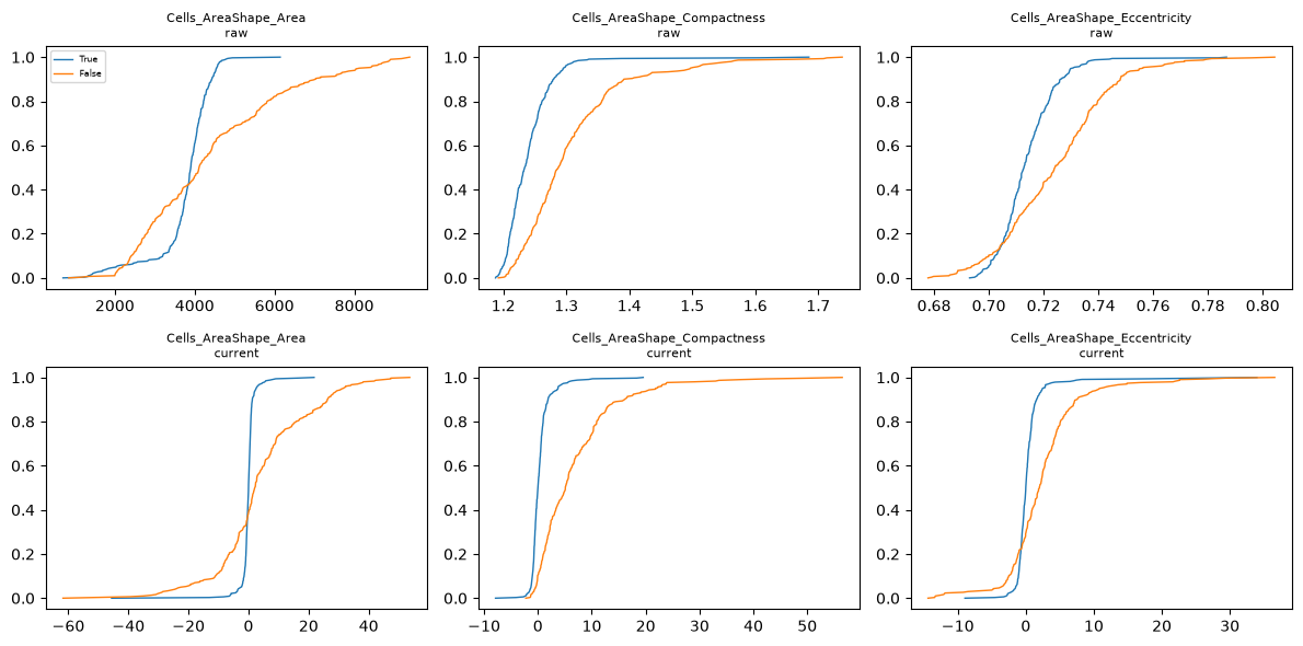
Before normalization each plate’s controls sit wherever that plate’s staining landed; after, the control wells are centred on zero by construction, and a treated well is read as its distance from that shared baseline. Every downstream distance is measured on this cleaned scale.
One profile per treatment#
Replicate wells of a treatment are noisy, and a screen is easier to reason about as one signature per treatment.
tl.consensus collapses replicates, taking the median by default (what pycytominer does).
signatures = mt.tl.consensus(treated, method="median", min_replicates=1)
signatures = signatures[signatures.obs["Metadata_MOA"].notna().to_numpy()].copy()
print(
    f"{treated.n_obs} treated wells -> {signatures.n_obs} treatment signatures"
    f" over {signatures.obs['Metadata_MOA'].nunique()} mechanisms"
)
302 treated wells -> 103 treatment signatures over 12 mechanisms
One row per treatment now, each the median of its replicate wells. These signatures are what the mechanism step compares.
What is a hit?#
A hit is a treatment whose profile moved away from the controls by more than the controls vary among themselves.
tl.hit_calling scores that distance in the controls’ own covariance and gives it a permutation p-value;
tl.effect_size then says which features moved.
mt.tl.hit_calling(adata, groupby="Metadata_Perturbation", use_rep="X_pca", n_permutations=1000)
mt.tl.effect_size(adata, groupby="Metadata_Perturbation")

hits = adata.uns["mantispy"]["hits"]
mt.pl.hits(adata)
mt.pl.feature_volcano(adata, group=hits.nlargest(1, "distance")["group"].iloc[0]);
Most treatments clear the threshold and the DMSO control does not: the assay separates active from inactive. The volcano for the strongest hit names the individual measurements carrying its phenotype, which is the handle for asking what the compound does.
One caveat before trusting a strong hit: a compound that kills most of the cells also moves the well median, for
reasons that are not the biology being screened. tl.cytotoxicity reads distance against viability so the two can
be told apart.
mt.tl.cytotoxicity(adata)
mt.pl.cytotoxicity(adata);
Groups in the upper left are far from the controls and have lost most of their cells: suspect, not necessarily biology. A large distance with intact viability is the hit worth following.
What does it do?#
Mechanism is a retrieval question: does a treatment’s nearest neighbour share its mechanism, and where the assay
fails, which mechanisms does morphology confuse? tl.nn_moa_classify with the not-same-compound rule (a compound
must be recognised from a different molecule with the same mechanism) answers the first.
mt.tl.nn_moa_classify(signatures, scheme="nsc")
mt.pl.moa_confusion(signatures);
The diagonal dominates: most treatments retrieve a different compound with the same mechanism. The largest off-diagonal block, Eg5 inhibitors against microtubule destabilizers, is biology (both arrest mitosis and look alike here) and not a failure of the classifier.
The whole map at once: tl.edistance gives every treatment-by-treatment distance, and pl.distance_heatmap
orders it by mechanism so related treatments form blocks on the diagonal.
mt.tl.edistance(signatures, reference=None)
mt.pl.distance_heatmap(signatures, groupby="Metadata_MOA");
Mechanism blocks stand out along the diagonal (compounds that share a mechanism sit close) while the off-diagonal shows which mechanisms the assay cannot separate. This is the same structure the confusion matrix summarised, now laid out treatment by treatment.
Everything is on the object#
Nothing above returned a result that lives only in a notebook variable. Hits and effect sizes are on adata, the
mechanism call is on signatures, and each result is a table under uns["mantispy"], beside the provenance of the
step that wrote it.
mt.io.write saves the object and every one of these tables in one .h5ad, and mt.io.read brings them back,
the same file a scanpy user can open.
Where to go next#
Each modality has its own tutorial that goes deeper than this page:
Compound screens, hits, effects and cell loss: activity, what moved, and whether a hit is a phenotype or dead cells.
Genetic screens, CRISPR knockouts: which knockouts have a phenotype, and whether the map recovers known biology.
Single cells, what the well median hides: the same questions asked below the well.
Across laboratories, cross-laboratory reproducibility: does the screen reproduce at another site.
How-to recipes, from a CellProfiler run and the other short data-loading examples.