Normalize, select, aggregate

Plates differ in imaging day, reagent lot and microscope state, and a CellProfiler run gives a few thousand features, most of them redundant. This page puts the cells of a JUMP plate on the scale of its own controls and aggregates them to wells, then reduces the features of a whole screen to the informative ones.

import matplotlib.pyplot as plt
import numpy as np

import mantispy as mt

cells = mt.ds.jump_cells()

import plotly.io as pio

pio.renderers.default = "notebook_connected"

Normalization

Plates differ in imaging day, reagent lot and microscope state. The standard fix is to express every cell relative to the negative controls on its own plate, which is what reference="negcon" together with by="Metadata_Plate" does.

The default method, mad_robustize, subtracts the control median and divides by a robust spread, so a few extreme cells do not set the scale.

mt.pp.normalize(cells, method="mad_robustize", by="Metadata_Plate", reference="negcon", keep_raw=True)

controls = cells[cells.obs["Metadata_Control"].to_numpy()]
np.round(np.nanmedian(np.asarray(controls.X), axis=0)[:5], 6)

array([0., 0., 0., 0., 0.], dtype=float32)

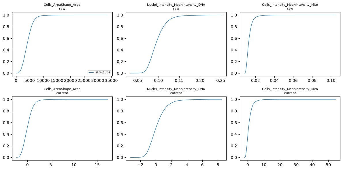
The controls now sit at zero on every plate by construction. keep_raw=True kept the original values in layers["raw"] for the before-and-after plot. It is off by default because the extra layer doubles memory and the original is already on disk.

mt.pl.feature_distributions(
    cells, features=["Cells_AreaShape_Area", "Nuclei_Intensity_MeanIntensity_DNA", "Cells_Intensity_MeanIntensity_Mito"]
);

Features normalization cannot scale

normalize warned about features in var["degenerate_scale"]. They have no spread among the control cells of some plate, so mad_robustize divides them by epsilon = 1e-18 instead of by zero, as pycytominer [Serrano et al., 2025] does, and multiplies them by up to 1e18.

{"flagged degenerate_scale": int(cells.var["degenerate_scale"].sum()), "of": cells.n_vars}

{'flagged degenerate_scale': 285, 'of': 5839}

A variance threshold does not catch a feature that varies across the plate and is constant among the control wells: it measures variance across all wells, keeps that feature, and the feature then dominates every distance computed afterwards. The flag catches it. feature_select() drops flagged features first by default and judges the rest without them. Anything that reads the object before selection needs them gone by hand:

adata = adata[:, ~adata.var["degenerate_scale"].to_numpy()].copy()

Aggregating to wells

Each well’s profile is the median across its cells. The median is used instead of the mean so that a few extreme cells do not move the profile.

wells = mt.tl.aggregate(cells, by=("Metadata_Plate", "Metadata_Well"), func="median")
wells

AnnData object with n_obs × n_vars = 24 × 5839
    obs: 'Metadata_Plate', 'Metadata_Well', 'Metadata_CellCount', 'Metadata_SiteCount', 'Metadata_BinningX', 'Metadata_BinningY', 'Metadata_ChannelID', 'Metadata_ChannelName', 'Metadata_Col', 'Metadata_ExposureTime', 'Metadata_ImageResolutionX', 'Metadata_ImageResolutionY', 'Metadata_ImageSizeX', 'Metadata_ImageSizeY', 'Metadata_MainEmissionWavelength', 'Metadata_MainExcitationWavelength', 'Metadata_MaxIntensity', 'Metadata_ObjectiveMagnification', 'Metadata_ObjectiveNA', 'Metadata_PlaneID', 'Metadata_PositionZ', 'Metadata_Row', 'Metadata_Source', 'Metadata_JCP2022', 'Metadata_InChIKey', 'Metadata_Perturbation', 'Metadata_Control'
    var: 'object', 'feature_group', 'feature', 'channel', 'scale', 'angle', 'gray_levels', 'radial_bin', 'params', 'is_feature', 'selected', 'degenerate_scale'
    uns: 'mantispy'
    layers: None (.X)

The result records its provenance and keeps every metadata column that is constant within a well. Columns that vary within a well, such as a per-cell measurement, are dropped because they have no single value per well.

wells.uns["mantispy"]["aggregated_from"]

{'by': ['Metadata_Plate', 'Metadata_Well'],
 'func': 'median',
 'n_obs': 13578,
 'min_cells': 10}

Metadata_CellCount is added as well. Cell count is a common confounder, and mt.pp.regress_out can remove its influence later.

Feature selection

Most of a CellProfiler run’s features are redundant. AreaShape_Area and AreaShape_Perimeter carry much the same information, and so does a texture feature at scale 3 and the same texture at scale 5. Others are constant, or blow up because they are ratios with a near-zero denominator. mantispy reproduces pycytominer’s operations [Serrano et al., 2025], verified feature by feature, because published pipelines depend on their precise behavior.

Selection needs a screen rather than one plate’s 24 wells. pki is the JUMP pilot’s kinase inhibitors: eight plates, 3,072 wells [Chandrasekaran et al., 2023].

screen = mt.ds.pki()
mt.pp.normalize(screen, method="mad_robustize", by="Metadata_Plate", reference="negcon")
screen

AnnData object with n_obs × n_vars = 3072 × 5839
    obs: 'Metadata_plate_map_name', 'Metadata_broad_sample', 'Metadata_mg_per_ml', 'Metadata_mmoles_per_liter', 'Metadata_solvent', 'Metadata_Plate', 'Metadata_Well', 'Metadata_Site_Count', 'Metadata_Count_Cells', 'Metadata_Count_CellsIncludingEdges', 'Metadata_Count_Cytoplasm', 'Metadata_Count_Nuclei', 'Metadata_Count_NucleiIncludingEdges', 'Metadata_Object_Count', 'Metadata_Barcode', 'Metadata_Supplier', 'Metadata_Supplier_Catalog', 'Metadata_pert_type', 'Metadata_control_type', 'Metadata_CellCount', 'Metadata_SiteCount', 'Metadata_Control', 'Metadata_Compound', 'Metadata_Concentration', 'Metadata_MOA', 'Metadata_Perturbation'
    var: 'object', 'feature_group', 'feature', 'channel', 'scale', 'angle', 'gray_levels', 'radial_bin', 'params', 'is_feature', 'degenerate_scale'
    uns: 'mantispy'
    layers: None (.X)

The operations

Each operation tests one criterion, and feature_select combines them. It does not drop anything: it writes a boolean column to var, and only subset_features changes the shape, so you can inspect what would be removed first.

operation	drops a feature when
drop_degenerate	normalize could not scale it and flagged it in var["degenerate_scale"]
variance_threshold	its variance is below min_variance
frequency_threshold	one value dominates it, or it takes very few distinct values
correlation_threshold	it is highly correlated with another feature
drop_na_columns	too much of it is missing
blocklist	it is on the CellProfiler blocklist of known-unreliable features
drop_outliers	its magnitude has blown up
noise_removal	it varies too much between replicates of the same perturbation

Two of these are easy to get wrong.

variance_threshold is a plain variance cut. The frequency-and-uniqueness rule often described under that name is a separate operation, frequency_threshold, and its two criteria combine with OR.

correlation_threshold uses the signed correlation, not the absolute value, so two features correlated at −1.0 are both kept. pycytominer does the same, and mantispy matches it.

for operation in ("drop_degenerate", "variance_threshold", "correlation_threshold", "drop_na_columns", "blocklist"):
    trial = screen.copy()
    mt.pp.feature_select(trial, operations=(operation,))
    print(f"{operation:24s} keeps {int(trial.var['selected'].sum()):5d} of {trial.n_vars}")

drop_degenerate          keeps  5706 of 5839
variance_threshold       keeps  5828 of 5839
correlation_threshold    keeps   928 of 5839
drop_na_columns          keeps  5839 of 5839
blocklist                keeps  5784 of 5839

Each operation is judged on its own here. correlation_threshold does the most, because most of a CellProfiler run is near-duplicates of other features.

Running the default pipeline

The default runs five of the eight operations: drop_degenerate, which runs first, and pycytominer’s own default of four. frequency_threshold and drop_outliers are off because both can remove an informative feature on a screen with few conditions, and noise_removal is off because it needs replicate structure, which not every object has.

mt.pp.feature_select(screen)
screen.uns["mantispy"]["feature_select"]

{'drop_degenerate': 133,
 'variance_threshold': 0,
 'correlation_threshold': 4836,
 'drop_na_columns': 0,
 'blocklist': 55}

Before and after

The correlation heatmap is ordered by feature group, with a line at each group boundary. Here it is for the shape measurements of the whole cell, before selection and after. Blocks along the diagonal are features that measure nearly the same thing.

shape = ((screen.var["object"] == "Cells") & (screen.var["feature_group"] == "AreaShape")).to_numpy()
fig, axes = plt.subplots(1, 2, figsize=(12, 5))
mt.pl.feature_correlation(screen[:, shape].copy(), key=None, ax=axes[0])
axes[0].set_title(f"before: {int(shape.sum())} features")
kept = shape & screen.var["selected"].to_numpy()
mt.pl.feature_correlation(screen[:, kept].copy(), key=None, ax=axes[1])
axes[1].set_title(f"after: {int(kept.sum())} features")
plt.show()

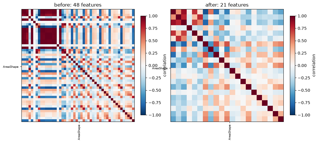
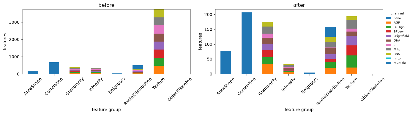
Of the 48 shape measurements of the whole cell, 21 survive. The large block of features that move together collapses to a few, and what remains correlates below the cutoff. Strongly negative pairs survive, because the cut uses the signed correlation, as pycytominer’s does. pl.feature_groups shows which feature families lost features to selection.

fig, axes = plt.subplots(1, 2, figsize=(14, 4))
mt.pl.feature_groups(screen, ax=axes[0])
axes[0].set_title("before")
mt.pl.feature_groups(screen, key="selected", ax=axes[1])
axes[1].set_title("after")
axes[0].get_legend().remove()  # both panels share the channels; one legend on the right is enough
fig.tight_layout()
plt.show()

Removing multivariate redundancy

correlation_threshold is pairwise: it drops one feature from each pair correlated above the cutoff. A feature that is a linear combination of several others, a texture that tracks the sum of two neighbouring scales, say, need not correlate strongly with any single one, so the pairwise cut keeps it even though it carries no new information.

decorrelate removes exactly that. A rank-revealing, column-pivoted QR [Businger and Golub, 1965, Golub and Van Loan, 2013] orders the features so that each is the one least explained by those already kept, and drops a feature once the features kept before it predict it at multiple correlation decorr_threshold. One decomposition does it, cheap enough to run at several strengths, and it keeps original features rather than projecting to components. It is experimental and not part of pycytominer, so it is opt-in via decorrelate=True.

How hard to decorrelate is a judgement call, so rather than trust one number, run it at a few thresholds and score each against the biological outcome you care about. Below: information retained, technical replicate retrieval, and biological activity retrieval (perturbation vs. control) [Kalinin et al., 2025].

import pandas as pd
from sklearn.linear_model import RidgeCV
from sklearn.model_selection import cross_val_predict

selected = mt.pp.subset_features(screen)  # the pycytominer set
reference = np.nan_to_num(np.asarray(selected.X, dtype=np.float64))
reference = (reference - reference.mean(0)) / (reference.std(0) + 1e-9)
rng = np.random.default_rng(0)


def information_kept(mask, n=30):
    """Cross-validated R2 predicting held-out pycytominer features from the kept subset."""
    block = reference[:, mask]
    scores = []
    for c in rng.choice(selected.n_vars, size=n, replace=False):
        y = reference[:, c]
        pred = cross_val_predict(RidgeCV(), block, y, cv=5)
        scores.append(1.0 - ((y - pred) ** 2).sum() / ((y - y.mean()) ** 2).sum())
    return round(float(np.mean(scores)), 3)


def retrieval(subset, mode):
    """Mean mAP over the treated wells: replicate (technical) or activity (biological) retrieval."""
    adata = subset.copy()
    mt.tl.map(adata, mode=mode, null_size=1000, seed=0, **({"reference": None} if mode == "replicability" else {}))
    treated = ~adata.obs["Metadata_Control"].to_numpy()
    return round(float(adata.obs["map"].to_numpy()[treated].mean()), 3)


rows, index = [], []
for threshold in [None, 0.99, 0.95, 0.9]:
    if threshold is None:
        subset, mask, label = selected, np.ones(selected.n_vars, bool), "exact"
    else:
        flagged = selected.copy()
        mt.pp.feature_select(flagged, operations=(), decorrelate=True, decorr_threshold=threshold)
        mask = flagged.var["selected"].to_numpy()
        subset, label = mt.pp.subset_features(flagged), f"decorrelate {threshold}"
    rows.append(
        {
            "features": subset.n_vars,
            "information kept (R2)": 1.0 if threshold is None else information_kept(mask),
            "replicate mAP": retrieval(subset, "replicability"),
            "activity mAP": retrieval(subset, "activity"),
        }
    )
    index.append(label)
pd.DataFrame(rows, index=index)

	features	information kept (R2)	replicate mAP	activity mAP
exact	850	1.000	0.219	0.632
decorrelate 0.99	518	0.980	0.216	0.615
decorrelate 0.95	272	0.925	0.212	0.603
decorrelate 0.9	180	0.842	0.213	0.603

decorrelate is a dial, and there is no free lunch: a lower threshold removes more features, but because the redundant ones still carry a sliver of unique signal, retrieval falls with them. The technical replicate retrieval is nearly flat here; the biological activity retrieval is the one that pays, gently at 0.99, where the set nearly halves, and more by 0.9. On a screen with real mechanism-of-action structure the trade is often kinder still, because dropping redundant, noisy features can tighten same-MOA neighbourhoods, but pki has too few compounds per MOA to show that here.

So the recommendation is the workflow above rather than a fixed cutoff: sweep a few thresholds, compare against the metric that matters for your screen, and keep the smallest set that still holds it. decorr_threshold=0.99 is a sensible place to start.

The blocklist

The default blocklist is pycytominer’s, copied unchanged with its source recorded in the file. It lists features known to be unreliable: twenty Manders and twenty rank-weighted colocalization coefficients, plus the three highest nuclear granularity bands in each channel. MeasureColocalization writes Manders, RWC and Costes coefficients, and only the first two are on the list.

from mantispy._core.features import load_blocklist

blocked = load_blocklist()
{"on the list": len(blocked), "in this screen": int(screen.var_names.isin(blocked).sum()), "examples": blocked[:3]}

{'on the list': 55,
 'in this screen': 55,
 'examples': ['Nuclei_Correlation_Manders_AGP_DNA',
  'Nuclei_Correlation_Manders_AGP_ER',
  'Nuclei_Correlation_Manders_AGP_Mito']}

Scaling correlation to large screens

correlation_threshold compares every pair of features, so its cost grows with the square of the feature count; on a screen with tens of thousands of features the exact pass takes minutes.

mantispy keeps the exact pass as the default, matching pycytominer [Serrano et al., 2025]. Passing corr_window switches to a faster two-pass approximation: pass one sorts features by name (a CellProfiler family sorts together) and prunes redundancy only within a sliding window, which is cheap and whittles the list down; pass two runs the exact all-pairs correlation on the survivors, a much smaller set, so it catches the cross-family redundancy the windows could not see while its quadratic cost stays small. A window of 500 is a good default.

Be clear about the deviation from the standard: the fast pass does not reproduce the exact pass feature for feature. Correlated features are near-duplicates, so which member survives is close to arbitrary, and the fast pass keeps a different set. What matters is whether the reduced space keeps the same information and the same biology. The next cells measure exactly that, across strategies.

import time

import numpy as np
import pandas as pd

# Normalize a copy so the downstream mAP is meaningful, then compare selection strategies on it.
base = screen.copy()
mt.pp.normalize(base, method="mad_robustize", by="Metadata_Plate")
matrix = np.nan_to_num(np.asarray(base.X, dtype=np.float64))
matrix = (matrix - matrix.mean(0)) / (matrix.std(0) + 1e-9)
rng = np.random.default_rng(0)


def reconstruct_r2(target, predictors, n=30):
    """Cross-validated R2 predicting each target feature from the predictor feature set."""
    # cross-validated R2 predicting each target feature from the predictor set: is the information kept
    cols = rng.choice(target, size=min(n, len(target)), replace=False)
    block = matrix[:, predictors]
    scores = []
    for c in cols:
        y = matrix[:, c]
        tot = ((y - y.mean()) ** 2).sum()
        if tot == 0:
            scores.append(1.0)
            continue
        pred = cross_val_predict(RidgeCV(), block, y, cv=5)
        scores.append(1.0 - ((y - pred) ** 2).sum() / tot)
    return float(np.mean(scores))


def select(**kwargs):
    """Run feature_select with these kwargs; return the boolean selection mask and the runtime."""
    adata = base.copy()
    start = time.perf_counter()
    mt.pp.feature_select(adata, operations=("drop_degenerate", "correlation_threshold"), **kwargs)
    return adata.var["selected"].to_numpy(dtype=bool), time.perf_counter() - start


def replicate_map(mask):
    """Mean replicate-retrieval mAP on the subset of features flagged by mask."""
    # downstream biology: do a compound's replicate wells retrieve each other in the reduced space
    adata = base[:, mask].copy()
    mt.tl.map(adata, mode="replicability", null_size=1000, reference=None, seed=0)
    return float(adata.obs["map"].mean())


strategies = {"exact": {}, "fast (window 500)": {"corr_window": 500}, "fast (window 1500)": {"corr_window": 1500}}
masks = {name: select(**kw) for name, kw in strategies.items()}
exact_mask = masks["exact"][0]
exact_idx = np.flatnonzero(exact_mask)

rows = []
for name, (mask, seconds) in masks.items():
    idx = np.flatnonzero(mask)
    rows.append(
        {
            "features kept": int(mask.sum()),
            "time (s)": round(seconds, 1),
            "overlap with exact (Jaccard)": round((exact_mask & mask).sum() / (exact_mask | mask).sum(), 3),
            "information kept (R2 vs exact)": 1.0 if name == "exact" else round(reconstruct_r2(exact_idx, idx), 3),
            "replicate mAP": round(replicate_map(mask), 3),
        }
    )
pd.DataFrame(rows, index=list(strategies))

	features kept	time (s)	overlap with exact (Jaccard)	information kept (R2 vs exact)	replicate mAP
exact	853	3.5	1.000	1.000	0.419
fast (window 500)	972	0.8	0.548	0.995	0.421
fast (window 1500)	988	1.1	0.551	0.991	0.420

Interpret the table you expect: the fast selections overlap the exact one only about half at the feature level (this is the deviation from pycytominer, and it is real), yet they reconstruct the exact features at an R2 near 1 and reach the same replicate mAP. Different features, same information, same biology. Window size trades a little speed for a slightly larger, still-equivalent set.

from anndata import AnnData

rng = np.random.default_rng(0)
n_cells, n_features, n_drivers = 2000, 20_000, 1500
drivers = rng.standard_normal((n_cells, n_drivers), dtype=np.float32)
assign = np.sort(rng.integers(0, n_drivers, size=n_features))
X = drivers[:, assign] + rng.standard_normal((n_cells, n_features), dtype=np.float32) * 0.05
names = [f"Cells_Texture_Driver{assign[i]:05d}_{i:06d}" for i in range(n_features)]
big = AnnData(X, var=pd.DataFrame(index=names))


def timed(**kwargs):
    """Run feature_select on the synthetic screen; return the runtime and the features kept."""
    adata = big.copy()
    start = time.perf_counter()
    mt.pp.feature_select(adata, operations=("correlation_threshold",), **kwargs)
    return time.perf_counter() - start, int(adata.var["selected"].sum())


exact_time, exact_kept = timed()
fast_time, fast_kept = timed(corr_window=500)
{
    "features": n_features,
    "exact": f"{exact_time:.1f}s, {exact_kept} kept",
    "fast (window 500)": f"{fast_time:.1f}s, {fast_kept} kept",
    "speedup": f"{exact_time / fast_time:.1f}x",
}

{'features': 20000,
 'exact': '23.0s, 1500 kept',
 'fast (window 500)': '1.8s, 1500 kept',
 'speedup': '12.7x'}

Guidance: use the exact default for faithful pycytominer parity, and reach for corr_window=500 when a screen has many thousands of features and the correlation step dominates. The saving grows with the feature count, and the reduced space carries the same information and the same replicate signal.

Looking at the plates

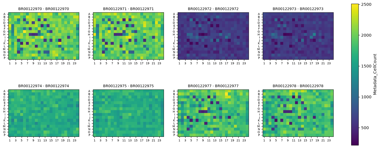
Plate layout artifacts are easiest to see on a plate map. pl.plate draws any feature or obs column; here, how many cells each well of the eight plates held.

mt.pl.plate(screen, color="Metadata_CellCount", groupby="Metadata_Plate", ncols=4);

Handing off

get.to_dataframe returns the flat, metadata-first table that pycytominer [Serrano et al., 2025], cytominer-eval and most published scripts expect.

frame = mt.get.to_dataframe(mt.pp.subset_features(screen))
frame.iloc[:3, :6]

	Metadata_plate_map_name	Metadata_broad_sample	Metadata_mg_per_ml	Metadata_mmoles_per_liter	Metadata_solvent	Metadata_Plate
0	C-7210-01-CMP-014	NaN	NaN	NaN	DMSO	BR00122970
1	C-7210-01-CMP-014	NaN	NaN	NaN	DMSO	BR00122970
2	C-7210-01-CMP-014	NaN	NaN	NaN	DMSO	BR00122970

Next: Plate artifacts and corrections.